Extensions of Karger's algorithm
If you prefer videos, check out our ICCV presentation, which covers similar content as this blog post. For more details, see our paper.
Karger’s contraction algorithm is a fast and very famous method for finding global minimum graph cuts. First published in 1993, it helped start a wave of other randomized algorithms for graph cut problems. And while many of these are asymptotically even faster, Karger’s algorithm remains important and fascinating in part because of its extreme simplicity – it’s description wouldn’t even require an entire postcard:
Contract a randomly chosen edge, i.e. merge the two nodes it connects into one node. Repeat until only two nodes are left.
We will discuss Karger’s algorithm in a bit more detail shortly. But first, this simplicity raises a question: can Karger’s algorithm be extended to help with other tasks than the global minimum cut problem it was originally meant to solve? That is the question we aim to answer in our new paper and which this blog post will focus on.
One extension that immediately suggests itself, and which we will discuss first, is that to \(s\)-\(t\)-mincuts. If you already know what \(s\)-\(t\)-mincuts are and why we’d want to find them, you can read on; if you’d rather have a brief refresher, there’s one in the expandable box below.
What are \(s\)-\(t\)-mincuts and why care about them?
\(s\)-\(t\)-mincuts (and the related max flows) play an enormously important role in computer science in general. But instead of giving a huge list, we’ll focus on just one application to computer vision: Say you have an image that you want to segment into fore- and background. You might have a neural network that can tell you how likely each pixel is to belong to either of these classes. But in the end, you don’t want all these numbers, you want a single “best guess” segmentation.
You could of course just assign each pixel to the more likely class: make a pixel part of the foreground whenever the network says it’s more likely to be foreground than background. But this would ignore dependencies between pixels: if there is a region where the network classifies most pixels as slightly more likely to be background but there are a few exceptions, then you probably don’t want these exceptions to be part of the foreground. We know that fore- and background are at least somewhat contiguous and we want to make use of this prior knowledge.
One approach to this is shown in the following figure:
, which in turn was adapted from [Boykov, Yuri and Funka-Lea, Gareth (2006)](https://link.springer.com/article/10.1007/s11263-006-7934-5).](/post/karger-extensions/st_cut_hu7a979f5552f8ad097f1d3740ca26fde1_102710_c8d59361788408cb2101b08b16c86667.webp)
We turn our image into a graph; each pixel becomes one of the gray nodes in the graph. Then we add two more nodes, \(s\) and \(t\) (in red and blue). They are “helper nodes” that represent the foreground and background. We add edges from each pixel node to both \(s\) and \(t\) and use the probabilities from our neural network to determine positive weights for these edges (for example, a probability of 0.5 would mean that the edge connecting that pixel to \(s\) has the same weight as the edge to \(t\)).
We also add edges between neighboring pixel nodes (the yellow edges in the figure). Their weights describe how similar two pixels are; they could just be calculated from brightness differences or they could come from an edge detector network.
The goal is now to cut this entire graph into two halves, one containing \(s\) and the other containing \(t\). And we want to do this in such a way that the total weight of all edges that are cut is as small as possible – strongly connected nodes should remain on the same side of the cut.
For each pixel, we will have to cut either its edge to \(s\) or to \(t\); this is where the probabilities predicted by the neural network come in. But we will also have to cut edges between pixels themselves, and this is what biases the segmentation towards one that doesn’t split up homogeneous areas of the image.
Global mincuts and Karger’s algorithm
Karger’s algorithm doesn’t find \(s\)-\(t\)-mincuts, it finds global minimum cuts. This means that we want to separate a graph into two parts while minimizing the total weight of edges that need to be cut – all without having seeds \(s\) and \(t\) that need to be separated.
The following figure illustrates how Karger’s algorithm works on a simple example graph: we first selects an edge at random, in this case the one between \(b\) and \(c\) (in red), and then contract the chosen edge. We then repeat this process until only two nodes are left (on the very right). These nodes define a cut of the original graph into the partitions \(\{a\}\) and \(\{b, c, d\}\).

This works for unweighted graphs and for graphs with positive edge weights (in which case edges are selected for contraction with probability proportional to their weight).
Since Karger’s algorithm uses random contractions, it could of course produce a different result on the same input graph, and in particular a non-minimal cut. But importantly, Karger’s algorithm produces a minimum cut with a reasonably high probability: by running it a polynomial number of times, it becomes very likely that at least one run will find a minimum cut. This is far from obvious: there can be an exponential number of cuts of a graph, so Karger’s algorithm needs a very strong bias towards minimum cuts to achieve its high success probability.
Karger’s algorithm for \(s\)-\(t\)-mincuts?
We can now come to our first question: can methods similar to Karger’s algorithm be applied to the \(s\)-\(t\)-mincut problem, rather than the global one?
It’s certainly easy to modify Karger’s algorithm such that it always separates \(s\) and \(t\): we simply never contract an edge that connects \(s\) and \(t\) (or nodes that \(s\) or \(t\) have been merged into). This will make sure that \(s\) and \(t\) are on opposite sides of the final remaining edge that defines the cut.
But unfortunately, we show that a wide class of extensions of Karger’s algorithm cannot find \(s\)-\(t\)-mincuts efficiently – no matter how clever we are in modifying Karger’s algorithm, there will always be some graphs where the success probability is exponentially low. Expand the box below if you want a few more details and intuition, or see the paper itself for all the gory details.
Karger’s algorithm can’t be extended to s-t-mincuts
Let’s start by understanding why it’s not enough to just slightly modify Karger’s algorithm such that it never merges \(s\) and \(t\). One kind of example where this simple algorithm fails is the following:

The \(s\)-\(t\)-mincut of this graph cuts all of the lighter edges (connected to \(t\)). For each of the parallel paths from \(s\) to \(t\), the Karger-based algorithm would choose either the heavy or the light edge for contraction at some point. It (correctly) chooses the heavy edge with probability \(2/3\), which sounds good at first. But its choices across all the paths are independent and so the probability that it gets all of them right and thus finds the \(s\)-\(t\)-mincut is only \((2/3)^n\), where \(n\) is the number of nodes besides \(s\) and \(t\). So the success probability of a single run is exponentially low and therefore, an exponential number of runs is needed to make success likely.
Ok, so perhaps we just need to be a bit more clever? For example, in the graph above, a greedy algorithm that always contracts the heaviest edge would work. It’s easy to construct counterexamples to that as well, but is there maybe some extension of Karger’s algorithm that does work for \(s\)-\(t\)-mincuts?
To make this question tractable, we need to be more precise about what “extensions of Karger’s algorithm” are. What we would like to keep is the basic structure of randomly selecting edges and then contracting them. That leaves one thing we can vary: how to calculate the probabilities with which each edge is chosen for contraction. We call algorithms with the basic structure of Karger’s algorithm but with arbitrary contraction probabilities (generalized) contraction algorithms.
So can generalized contraction algorithms solve the \(s\)-\(t\)-mincut problem? The answer is in fact yes! But don’t get excited because it’s very impractical: we can compute an \(s\)-\(t\)-mincut using some other algorithm and then set the contraction probability of all edges that are part of this mincut to 0. This way, we will always find an \(s\)-\(t\)-mincut. But of course this only shows that the framework of generalized contraction algorithms is too broad for our purposes, because we certainly don’t want to include silly choices such as this.
Let’s therefore consider two natural subclasses of contraction algorithms:
- local contraction algorithms compute contraction probabilities based only on a neighborhood of each edge and on global properties of the entire graph. Think of it like this: to assign a probability to an edge \(e\), you may look at a small neighborhood of \(e\) and at the entire graph, but you won’t be told which of the edges in this graph is \(e\).
- continuous contraction algorithms can make use of global properties of edges, but the probabilities they compute have to be a continuous function of the edge weights of the graph. So if the weights are perturbed only slightly, then all of the contraction probabilities may only change slightly as well.
Karger’s algorithm and its simple extension to \(s\)-\(t\)-cuts we described above are both local and continuous, as are many other reasonable extensions.
For these large classes of contraction algorithms, we can answer the question from above: they cannot solve the \(s\)-\(t\)-mincut problem efficiently in general – we can find graphs on which their success probability is exponentially low, meaning they would need to be run an exponential number of times.
For the full proofs (and the formal definitions of local and continuous contraction algorithms), see our paper. If you are only interested in the proof ideas, you can also expand the box below (yes, a box within a box!).
Proof ideas
For the impossibility result for local contraction algorithms, the idea is similar to what we already used to show that the simplest extension of Karger’s algorithm has an exponentially low success probability: we have a graph with many parallel paths between \(s\) and \(t\), all of which have to be independently contracted. The tricky part is designing these in such a way that no local algorithm can tell which edges to contract and which edges not to contract. We can’t simply have linear paths, instead we need to have broader “bands”. Each of these bands consists of somewhere between 9 and 18 nodes (rather than just one node as in the graph above), but other than that, the idea is the same.
The version for continuous contraction algorithms uses a very different but simple idea: start with a graph that has an exponential number of \(s\)-\(t\)-mincuts. Then there must be at least one cut that the algorithm assigns exponentially low probability to. Now slightly perturb the graph to make this cut the unique \(s\)-\(t\)-mincut. The probability of finding it will then remain extremely low because of the continuity condition.
By the way, these results also hold for normalized cuts (another important type of graph cut problem). We’ve chosen to focus on \(s\)-\(t\)-mincuts in this post purely because they are a bit simpler to define and more well-known, but the impossibility results hold for both cut problems (and even with similar proofs).
Karger’s algorithm for seeded segmentation
So far, extending Karger’s algorithm doesn’t look promising. But it turns out that there are useful extension of Karger’s algorithm – we just have to switch problems. Instead of a minimum cut, machine learning often requires a “good” segmentation in a vaguer sense – something that leads to good downstream performance. So that’s what we’ll tackle next.
To keep things simple in this blog post, let’s assume that our segmentation problem has only two classes, fore- and background, and that there is only one seed in each class.1 We’ll continue to call these seeds \(s\) and \(t\) and still want to separate them, we just don’t want a minimum cut any longer.
We could find a segmentation of the graph by just running Karger’s algorithm once and taking the cut we get that way. But that’s a bad idea: it’s extremely noisy and the individual cuts that Karger’s algorithm produces are often not good segmentations.
So instead, we sample a lot of cuts and then take their “mean”. Mre precisely: we generate an ensemble of cuts using the variation of Karger’s algorithms that never merges the two seeds. Then for each node \(v\), we count how often it ended up on the same side of the cut as \(s\) and how often on the \(t\) side. We can define the probability \(p_{\text{karger}}(v)\) that Karger’s algorithm puts \(v\) on the side of \(s\); our finite ensemble thus gives us an estimate of this probability.
This is illustrated in the following figure: displayed are six cuts that Karger’s algorithm might produce for different runs on the same graph. \(v\) is on the red side of the cut, the one belonging to \(s\), five out of six times, so we would estimate \(p_{\text{karger}}(v) \approx 5/6\). In practice, we of course use more than six runs.


This probability \(p_{karger}(v)\) is a probabilistic segmentation of the input graph. The following figure illustrates this and compares it to the potential that the random walker algorithm produces:
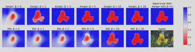
\(\beta\) is a parameter that influences how the edge weights are computed based on the image. For large \(\beta\), the edge weights become very extreme and both algorithms assign probabilities close to zero or one to each pixel.
If we need a hard cut, we can simply assign each pixel to the side for which this estimate is higher. This gives an algorithm for seeded graph segmentation. It’s very simple and has a great asymptotic runtime (linear in the number of edges of the graph). We also empirically compared this Karger-based segmentation method to the random walker and other algorithms on image segmentation and semi-supervised classification tasks. In both cases we found that it performs at least as well as these classical algorithms, see the paper for detailed results.
Karger’s algorithm and the random walker
We didn’t compare the Karger-based segmentation algorithm to the random walker just because the latter is one of the most influential algorithms for seeded segmentation of all time: it turns out that these two very different-seeming algorithms are surprisingly similar from a theoretical perspective.
Explaining these similarities takes some setup, so here’s the TL;DR: both algorithms can be interpreted as forest-sampling methods, just sampling from different distributions. The Karger distributions contains an additional dependency on the topology of the graph, which we think makes it more “confident” (i.e. it assigns probabilities closer to zero and one).
If this summary has whetted your appetite, then we encourage you to expand the box below for details.
The connection between Karger’s algorithm and the random walker
First, if you’re not already familiar with the random walker and spanning forests, you can find a brief crash course in the following box-within-a-box:
Random walker and spanning forests refresher
The random walker algorithm solves the same problem as our Karger-based algorithm: given a graph with some seeds, assign labels to the remaining nodes. Again, we will focus on the case with only one foreground and one background seed.
The idea is simple and elegant: to assign a label to some node \(v\), imagine a random walk starting at \(v\). At each step, we randomly move to one of the neighbors of the current node, with probability proportional to the weight of the edge connecting the nodes. The random walk stops once we reach one of the two seeds. We can define the probability \(p_{\text{rw}}(v)\) that this walk starting at \(v\) will end at the foreground seed. Just like the Karger-based algorithm, we thus get a probabilistic assignment for each node, and we can again get a hard segmentation by assigning each node to the more likely class.
So apart from the fact that they solve the same type of problem, why is the random walker relevant to us? To answer this question, let’s make yet another excursion, namely to forests and how they relate to segmentation. (I promise this will all circle back to Karger’s algorithm soon). A forest of a graph is a set of disjoint trees (i.e. acyclic connected graphs) that together span the entire graph. For example, in the following figure, the red edges define a 2-forest of the graph, i.e. a forest consisting of two trees:

In a seeded graph, we are particularly interested in forests that separate the seeds, which in our setting just means 2-forests such that \(s\) and \(t\) are in different trees. In the figure below, the forest on the left separates the seeds but the forest on the right does not:

A forest that separates the seeds automatically defines an assigment for each node – exactly what we’re after! One of the two trees will be the foreground and one will be the background:

In this figure, the colored edges are the tree; all nodes are colored according to the assigment defined by that tree.
Now comes the connection to the random walker: we can define a distribution over these 2-forests that separate the seeds, where the probability of a forest \(f\) consisting of edges \(e_1, \ldots, e_k\) is proportional to \[w(f) := \prod_{i = 1}^k e_i,\] called the weight of the forest. Then it turns out – this is not at all obvious – that the random walker probability \(p_{\text{rw}}(v)\) defined previously is exactly the probability that a forest sampled from this distribution assigns \(v\) to the foreground! So the random walker could be interpreted completely differently as a forest sampling method. In principle, we could sample lots of forests from this Gibbs distribution and then counting how often each node is assigned to each seed. Now, implementing the random walker like that would be computationally nonsensical – but it does sound notably similar to our Karger-based algorithm. (I promised we’d get back there).
The key insight to see the connection between the random walker and Karger’s algorithm is the following:
Karger’s algorithm samples spanning forests.
Essentially, the \(n - 2\) edges that Karger’s algorithm contracts during one run define a spanning 2-forest of the graph. And if we modify Karger’s algorithm such that it never merges \(s\) and \(t\), then this forest will separate \(s\) and \(t\). Furthermore, the two trees making up the sampled forest are precisely the two sides of the cut produced by Karger’s algorithm.
Details for curious readers
Some care needs to be taken here: the way we described Karger’s algorithm above, the edges it contracts may be the product of combining several edges of the original graph (because parallel edges are combined at each step). But as long as we don’t mind dealing with multigraphs, we can formulate a completely equivalent version of Karger’s algorithm that doesn’t combine parallel edges. This variation of Karger’s algorithm has exactly the same probability of producing any given cut as our formulation above. The only difference is that a run of this algorithm corresponds one-to-one to an ordered sequence of \(n - 2\) edges in the original graph.
Now it’s easy to prove that these \(n - 2\) edges always form a spanning 2-forest of the graph. We only need to note that this set of edges cannot contain any cycles because such cycles would correspond to self-loops in the contracted graph and the edge that closes the cycle would have been removed before it could be contracted.
The remaining difference between this Karger-based algorithm and the random walker is the distribution over forests that they sample from. Recall that for the random walker, the probability of sampling a forest \(f = (e_1, \ldots, e_{n - 2})\) is simply proportional to the weight \(w(f)\) of the forest. The distribution that Karger’s algorithm implicitly samples from also contains this term, but it has an additional dependency on the forest. It assigns a probability of \[ p(f) = w(f) \sum_{\sigma \in S_{n - 2}} \prod_{i = 1}^{n - 2} \frac{1}{c\left(E \setminus \mathcal{C}(\{e_{\sigma(1)}, \ldots, e_{\sigma(i - 1)}\})\right)} \] to a forest \(f = (e_1, \ldots, e_{n - 2})\). Understanding this equation is not important for the remainder of this post; you can find some details below and the full derivation in our paper.
Details on the Karger distribution
This equation is best understood starting from the right. \(E\) is simply the set of edges in the graph. \(\mathcal{C}(\hat{E})\) for a subset \(\hat{E} \subseteq E\) of edges is the set of all edges that together with \(\hat{E}\) form cycles or a connection between \(s\) and \(t\), as well as the edges in \(\hat{E}\) itself. These are precisely the edges that have been removed from the graph after contracting all the edges in \(\hat{E}\). \(c(\hat{E})\) is the sum of all the edge weights of edges in \(\hat{E}\). The fraction on the right side is therefore the normalization constant appearing in the probability of contracting any given edge. Taking the product over these (together with the weight \(w(f)\)) gives the probability of a particular run of Karger’s algorithm. A run corresponds to an ordered sequence of edges, whereas the ordering doesn’t matter for the forest defined by the run. So we need to sum over the set \(S_{n - 2}\) of all possible permutations of \(1, \ldots, n - 2\).
As we argue in the paper, this additional term makes the Karger potential more “confident” than the random walker potential, in the sense that it assigns more extreme probabilities to each node. This can also be seen in the plot of the potentials for an image we had above.
Conclusion
Karger’s algorithm is a powerful and very influential tool for finding global minimum cuts, so it is natural to ask whether this success can be extended to other important graph problems. We have proven that extending it to the \(s\)-\(t\)-mincut problem is impossible in a formal sense. However, we did adapt Karger’s algorithm to the problem of seeded graph segmentation, demonstrating its usefulness beyond minimum cuts. In particular, the new algorithm shows that the distribution produced by Karger’s algorithm is itself an interesting subject of study, rather than only the smallest cut found. We have made some steps towards understanding this distribution by linking it to the random walker. But there certainly remains a lot of space to improve our theoretical understanding of the “Karger distribution”, as well as the potential to use it for other purposes than the one we presented.
-
Generalizing to many classes and many seeds per class is straightforward, see our paper. ↩︎