L1 regularization: sparsity through singularities

Additive $L_1$ or $L_2$ penalties are two common regularization methods and their most famous difference is probably that $L_1$ regularization leads to sparse weights (i.e. some weights being exactly 0) whereas $L_2$ regularization doesn’t. There are many pictures and intuitive explanations for this out there but while those are great to build some understanding, I think they conceal the arguably deeper reason why $L_1$ regularization leads to sparse weights. But before we discuss that, we need to understand why $L_2$ regularization does not help to get sparse weights.

$L_2$ regularization doesn’t lead to any sparsity

Let $w$ be a vector of parameters and $\mathcal{L}(w)$ be any continuously differentiable loss function¹. For $L_2$ regularization, we want to find

This means that the gradient has to be zero:

or in components:

So we can get $w_i = 0$ as the optimal solution only if $\frac{\partial \mathcal{L}}{\partial w_i}\big\rvert_{w_i = 0} = 0$, i.e. if $w_i = 0$ is already optimal without regularization! So $L_2$ regularization doesn’t help to get sparsity at all. The same is true for $L_p$ regularization for any $p > 1$, because

$L_1$ regularization: non-differentiability to the rescue

$L_1$ regularization just uses the 1-norm instead of the Euclidean norm:

How does that change things? Well, the 1-norm of a vector is not differentiable at 0. More precisely:

So when can $w_i = 0$ be a local minimum of the regularized loss? We can’t just set the derivative to zero as before, because the derivative doesn’t exist.

To understand what we can do instead, let’s first recall why setting the derivative to zero works for differentiable functions. If $f(x)$ has a local minimum at 0, then this means that $f(x) \geq f(0)$ for all sufficiently small $x$. Since we assumed $f$ to be differentiable at $0$, $f(x)$ is well approximated² by

for small $x$. So if $f'(0) > 0$, then $f(x) < f(0)$ for small negative $x$, and if $f'(0) < 0$ we get the same for positive $x$. So the derivative at the minimum has to be zero, because otherwise taking a small step in the right direction would decrease the value.

We can apply the same idea to the loss with $L_1$ regularization: what happens if we take a small step $h$ away from $w_i = 0$? The loss is differentiable and thus changes approximately linearly:

But for the regularization term, the change is always just $|h|$, instead of a linear term:

So if we write $\tilde{\mathcal{L}}$ for the regularized loss, then we get

As long as $\left|\frac{\partial\mathcal{L}}{\partial w_i}\right| < \beta$, this is larger than the regularized loss at $w_i = 0$, because the $+ \beta |h|$ term will dominate. That is why $L_1$ regularization leads to sparser weights: it pulls all those weights to zero whose partial derivative at 0 has absolute value less than $\beta$³.

Interlude: Priors

If the loss function $\mathcal{L}$ models some log-likelihood, then regularization can be interpreted as performing maximum a posteriori (MAP) estimation rather than maximum likelihood estimation (MLE). This means we start with some prior over possible values of the parameter $w$, update this distribution using the evidence from the loss function, and then pick the parameters which are the most probable according to the posterior distribution.

$L_2$ regularization corresponds to a Gaussian prior and $L_1$ regularization to a Laplace prior (in both cases centered around 0). So it’s natural to try to explain the sparsity behavior of these regularization methods in terms of the underlying priors.

Here’s what a Gaussian (red) and Laplace (blue) distribution look like, both with unit variance and properly normalized:

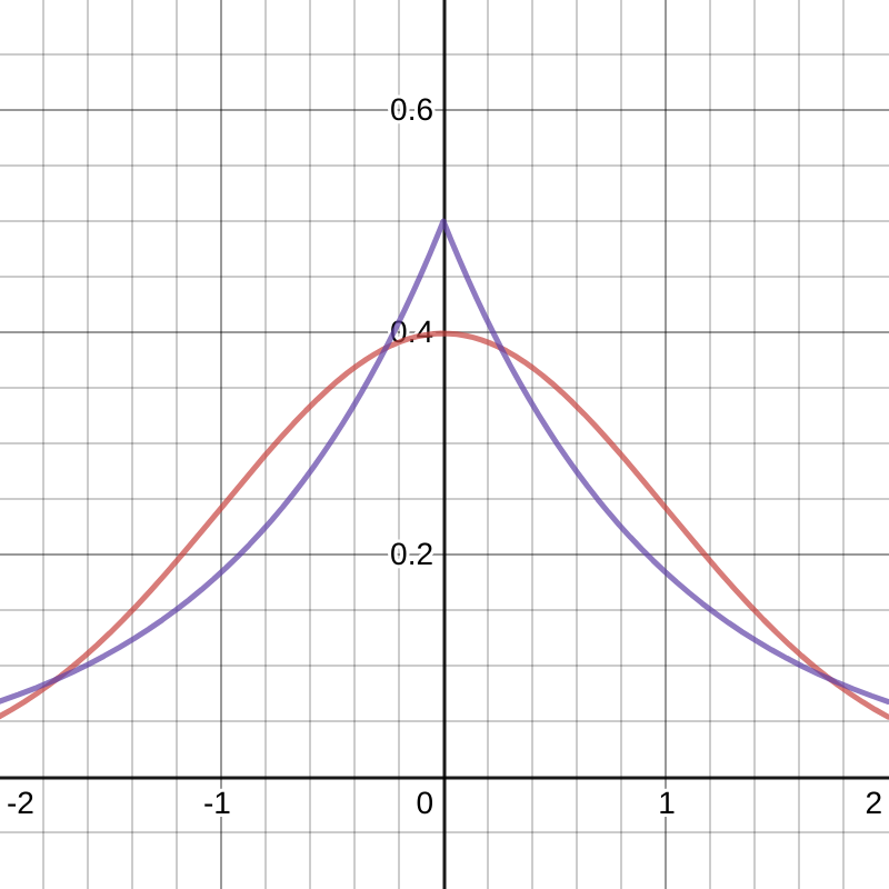
One difference is that the Laplace distribution has a higher density at (and around) 0. I’ve seen this used as an explanation for sparsity several times: the Laplace distribution seems more “concentrated” around 0, i.e. assigns a higher prior to 0, which is why we get sparse solutions.

But that is very misleading (and depending on what is meant by “concentrated” just wrong). Consider the following figure:

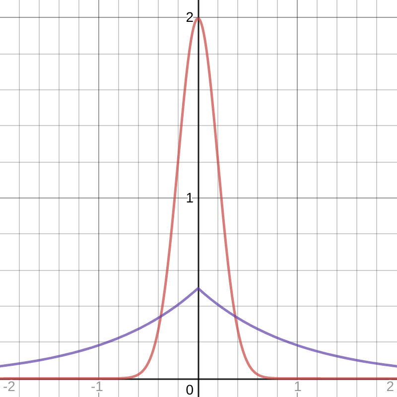
These are still a normalized Gaussian and a Laplace distribution, the only difference is that I’ve chosen a much smaller variance for the Gaussian. This corresponds to choosing a higher coefficient $\beta$ for the $L_2$ penalty. I’d argue that in this case the Gaussian is much more “concentrated around 0”, at least its density is much higher. But even with arbitrarily high $\beta$, $L_2$ regularization won’t lead to sparse solutions: you can make the prior as narrow as you like, and you’ll get weights that are closer and closer to zero but never precisely.

The real difference is the singularity (i.e. non-differentiability) of the Laplace distribution at 0. Since the logarithm is a diffeomorphism, singularities of the prior correspond 1-to-1 with singularities of the log prior, i.e. the regularization term.

Singularities are necessary for sparsity

We’ve seen that the difference between $L_1$ and $L_2$ regularization can be explained by the fact that the $L_1$ norm has a singularity while the $L_2$ norm doesn’t, or equivalently that the Laplace prior has one while the Gaussian prior doesn’t.

But we can say more than that: a singularity is in fact unavoidable if we want to make sparse weights likely. If we choose any continuously differentiable prior $p$ (or any continuously differentiable additive regularization term), then the overall objective $\tilde{\mathcal{L}}$ is continuously differentiable and therefore, the gradient has to be zero at a local minimum. So for $w_i = 0$ to be a local minimum, we’d need

which puts an equality constrain on $\frac{\partial \mathcal{L}}{\partial w_i}$: we only get sparse weights if the gradient has precisely the right value. Typically, this will almost surely not happen (in the mathematical sense, i.e. with probability 0), so non-singular regularization won’t lead to sparse weights.

In contrast, we saw that the singularity of the $L_1$ norm (or the Laplace prior) creates an inequality constraint for the partial derivative: it leads to $w_i = 0$ as long as the derivative lies in a certain range of values. This is what makes sparse weights likely.